This is Megatron
Megatron is a Python module for building data pipelines that encapsulate the entire machine learning process, from raw data to predictions.
The advantages of using Megatron:
- A wide array of data transformations can be applied, including:
- Built-in preprocessing transformations such as one-hot encoding, whitening, time-series windowing, etc.
- Any custom transformations you want, provided they take in Numpy arrays and output Numpy arrays.
- Sklearn preprocessors, unsupervised models (e.g. PCA), and supervised models. Basically, anything from sklearn.
- Keras models.
- To any Keras users, the API will be familiar: Megatron’s API is heavily inspired by the Keras Functional API, where each data transformation (whether a simple one-hot encoding or an entire neural network) is applied as a Layer.
- Since all datasets should be versioned, Megatron allows you to name and version your pipelines and associated output data.
- Pipeline outputs can be cached and looked up easily for each pipeline and version.
- The pipeline can be elegantly visualized as a graph, showing connections between layers similar to a Keras visualization.
- Data and input layer shapes can be loaded from structured data sources including:
- Pandas dataframes.
- CSVs.
- SQL database connections and queries.
- Pipelines can either take in and produce full datasets, or take in and produce batch generators, for maximum flexibility.
- Pipelines support eager execution for immediate examination of data and simpler debugging.
Installation
To install megatron, just grab it from pip:
pip install megatron
There’s also a Docker image available with all dependencies and optional dependencies installed:
docker pull ntaylor22/megatron
Tutorial
Let’s build the following pipeline:
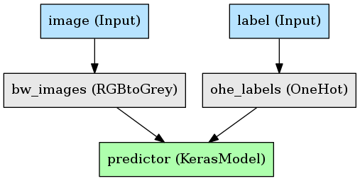
A simple example with an image and some binary labels. The goals here are:
- Convert the RGB image to black and white.
- One-hot encode the labels.
- Feed these into a Keras CNN, get predictions.
Let’s assume a built and compiled Keras model named “model” has already been made:
model = Model(image_input, two_class_output)
Let’s start by making the input nodes for the pipeline:
images = megatron.nodes.Input('image', (48, 48, 1))
labels = megatron.nodes.Input('label')
The first argument is a name, which is a mandatory argument for Inputs.
As for the second argument, by default, the shape of an Input is a 1D array, so we don’t need to specify the shape of ‘label’, but we will for ‘image’, which has a particular shape. The shape does _not_ include the first dimension, which is the observations.
Now let’s apply greyscaling to the image, and one-hot encoding to the labels:
grey_images = megatron.layers.RGBtoGrey(method='luminosity', keep_dim=True)(images)
ohe_labels = megatron.layers.OneHotRange(max_val=1)(labels)
4 things to note here:
- Calling a Layer produces a Node. That means Layers can be re-used to produce as many Nodes as we want, though we’re not taking advantage of that here.
- The initialization arguments to a Layer are its “hyperparameters”, or configuration parameters, such as the method used for converting RGB to greyscale.
- The first argument when calling a Layer is the previous layers you want to call it on. If there’s multiple inputs, they should be provided as a list.
- The second argument is the name for the resulting node. If this node is to be an output of the model, it must be named; otherwise, names are not necessary, though still helpful for documentation.
With our features and labels appropriately processed, we can pass them into our Keras model:
preds = megatron.layers.Keras(model)([grey_images, ohe_labels])
Since this is an output of the pipeline, we name it. Lastly, let’s attach a metric to the Keras model so we know how well it did:
acc = megatron.metrics.Accuracy()([ohe_labels, preds])
Note that metrics do not behave like other layers; they are not executed when we fit or transform. They come into play if we evaluate a Pipeline, at which point all the pipeline’s metrics will be calculated and given back to us. We’ll see that in a second.
To be able to identify the different metrics, it’s required that we name them, as the second argument to the call.
Finally, let’s create the pipeline by defining its inputs and outputs, just like a Keras Model:
storage_db = sqlite3.connect('getting_started')
pipeline = megatron.Pipeline([images, labels], preds, name='getting_started', version=0.1, storage=storage_db)
Let’s break down the arguments here:
- The first argument is either a single node or a list of nodes that are meant to be input nodes; that is, they will have data passed to them.
- The second argument is either a single node or a list of nodes that are meant to be output nodes; that is, when we run the pipeline, they’re the nodes whose data we’ll get.
- The pipeline must be named, and it can have a version number, but that is optional. These identifiers will be used for caching processed data and the pipeline itself.
- You can store the output data of a pipeline in a SQL database, and look it up using the index of the observations. If no index is provided (we provided no index here), it’s simply integers starting from 0.
Now let’s train the model, get the predictions, then lookup the prediction for the first observation from the storage database:
data = {'images': np.random.random((1000, 48, 48, 3)),
        'labels': np.random.randint(0, 1, 1000)}
pipeline.fit(data)
outputs = pipeline.transform(data)
one_output = pipeline.storage.read(rows=['0'])
print(outputs[0].shape) # --> (1000, 2)
print(one_output[0].shape) # --> (1, 2)

metrics = pipeline.evaluate(data)
print(metrics['model_acc']) # --> 0.51
What did we learn here?
- We pass in data by creating a dictionary, where the keys are the names of the input nodes of the pipeline, and the values are the Numpy arrays.
- Calling .transform(data) gives us a dictionary, where the keys are the names of the output nodes of the pipeline, and the values are the Numpy arrays.
- Looking up observations by index in the storage database gives us a dictionary with the same structure as .transform(data).
- Metrics are calculated by calling .evaluate(data) on the pipeline.
Finally, let’s save the pipeline to disk so it can be reloaded with its structure and trained parameters. Let’s save it under the directory “pipelines/”, from the current working directory:
pipeline.save('pipelines/')
The pipeline has been saved at the following location: [working_directory]/pipelines/getting_started-0.1.pkl. The name of the pickle file is the name of the pipeline and the version number, defined in its initialization, separated by a hyphen.
Let’s reload that pipeline:
pipeline = megatron.load_pipeline('pipelines/getting_started-0.1.pkl', storage_db=storage_db)
We provide the filepath for the pipeline we want to reload, and one extra argument: since we can’t pickle database connections, when we want to connect to the storage database, we have to make that connection variable and pass it as the second argument to load_pipeline. If you aren’t using caching, you don’t need to do this.
To summarize:
- We created a Keras model and some data transformations.
- We connected them up as a pipeline, ran some data through that pipeline, and got the results.
- We stored the results and the fitted pipeline on disk, looked up those results from disk, and reloaded the pipeline from disk.
- The data and pipeline were named and versioned, and the observations in the data had an index we could use for lookup.
Custom Layers
If you have a function that takes in Numpy arrays and produces Numpy arrays, you have two possible paths to adding it as a Layer in a Pipeline:
- The function has no parameters to learn, and will always return the same output for a given input. We refer to this as a “stateless” Layer.
- The function learns parameters (i.e. needs to be “fit”). We refer to this as a “stateful” Layer.
Custom Stateful Layers
To create a custom stateful layer, you will inherit the StatefulLayer base class, and write two methods: fit (or partial_fit), and transform. Here’s an example with a Whitening Layer:
class Whiten(megatron.layers.StatefulLayer):
    def fit(self, X):
        self.metadata['mean'] = X.mean(axis=0)
        self.metadata['std'] = X.std(axis=0)

    def transform(self, X):
        return (X - self.metadata['mean']) / self.metadata['std']
There’s a couple things to know here:
- When you calculate parameters during the fit, you store them in the provided dictionary self.metadata. You then retrieve them from this dictionary in your transform method.
- If your Layer is one that can be fit iteratively, you can override partial_fit rather than fit. If your transformation cannot be fit iteratively, you override fit; note that Layers without a partial_fit cannot be used with data generators, and will throw an error in that situation.
- For an example of how to write a partial_fit method, see megatron.layers.shaping.OneHotRange.).
Custom Stateless Layers
To create a custom stateless Layer, you can simply define your function and wrap it in megatron.layers.Lambda. For example:
def dot_product(X, Y):
    return np.dot(X, Y)

dot_xy = megatron.layers.Lambda(dot_product)([X_node, Y_node], 'dot_product_result')
That’s it, a simple wrapper.